All you need to know about: The Artificial Neural Networks (Part - 2)

(Reading time: 5 min)

The Plot of a Cost Function

A breakthrough in machine learning would be worth ten Microsofts.

-Bill Gates

Deep Neural Networks have proved to be an important tool for various applications in industry and academia. Machines have started to learn many things now, even better than humans.  In the previous post, we discussed the basics of neural networks. We learned how the weights and biases are assigned and how the decision boundary is manipulated by adding neurons or hidden layers. However, the most important (and the most interesting) component of 'an artificial brain' is its ability to learn. So in this article, we will study the concept of backpropagation and see how the learning process takes place. We will also assert the importance of large data in training and checking the performance of our neural network. 

Backpropagation

In supervised learning, we have a large labeled data which our neural network makes use of to train. We provide this data as input and assign random weights and biases. Because of these random parameters, we get an output at the end of the operation which is usually never accurate. This is where we make the network learn. A cost function is now defined which returns a high value whenever our predictions are way incorrect as compared to the actual value. Usually mean squared function is suited as the best choice for this purpose given by,

\(L = \frac{1}{2n}||y_{pred} - y_{actual}||^2\)

where \(L\) is the computed loss or cost, \(y_{pred}\) is the predicted value by our network, and \(y_{actual}\) is the actual value taken from the dataset. Predicting the value of the Loss function is not novel to just Neural Networks. Almost all the algorithms in Machine Learning (for e.g. KNN, Logistic Regression, etc) make use of cost function. The final goal of any machine learning model is to reduce or minimize the cost function. 

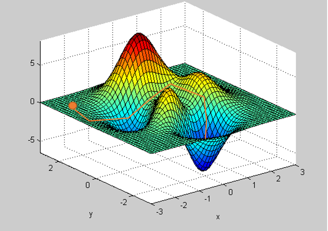
To minimize the cost, the weights, and biases of our network get adjusted to fit the training data in the best possible manner. This is achieved by employing gradient descent. 

One dimensional example of gradient descent

In gradient descent (as shown above), we have to minimize the cost function in a definite step size to attain the global minima. This can be achieved by introducing the derivative of the cost function for all the weights into our equation of updated weights for every single iteration. The equation for it is given by:

\(\Delta w_j = -\eta \frac{\partial J}{\partial w_j}\)

where \(\Delta w_j\) is the change in the weight needed to be done to minimize the cost, \(\eta\) is the learning rate (greater the learning rate, faster our network will converge to the result but with some disadvantages) and here \(J\) is the cost function. The equation for this updated weight is given as follows:

\(\textbf{w} = : \textbf{w} + \Delta \textbf{w}\)

Consider a neural network with 2 hidden layers. Once the learning process initiates, the weights in the structure start to change in a way to optimize the output. Consider our network is trying to update the weight shown in red. As it is clearly evident, any changes in that weight (or any weight in particular) are going to change the values in the subsequently hidden neurons and that will, in turn, change the output. The deeper the weight in which the change is introduced, the greater is the impact on the output. 

The equation for this follows the chain rule update as follows:

\(\frac{\partial J}{\partial w_j} = \frac{\partial J}{\partial w_0} \frac{\partial w_0}{\partial w_1} \frac{\partial w_1}{\partial w_2}...\frac{\partial w_{j-1}}{\partial w_j}\)

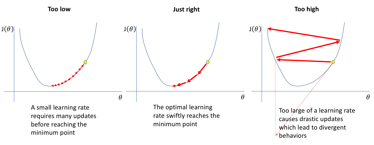
For many iterations throughout the process (also called Epochs), this procedure is repeated for a given training dataset so that we get a fully trained network giving us the best possible results. It is also crucial to talk about the learning rate \(\eta\). Since we are trying to optimize the network (trying to minimize the cost), we are essentially looking for the global minimum. Achieving this minimum requires us to specify the step size with which our algorithm proceeds. If we set our workflow such that very tiny changes are introduced for every change in weights and biases (as shown in the below figure on the left), it will take us a lot of time to reach our goal. This is theoretically the best approach as far as getting a good model is concerned, however computational too costly and thus not practical. If the alteration in wights and biases makes our result change dramatically, there's a high chance that our result may never converge (rightmost figure below). The image in the middle is the best possible way one can proceed to get the best result which is computationally feasible. 

Effect of Different Learning rates (step-sizes) while training

Since we are talking about supervised learning here, the size of the dataset plays a useful role as the larger the data, the greater is the ease with which our neural network is going to perform and understand the underlying pattern. A great combination of step-size and size of data is useful in making our model less prone to over and underfitting. Underfitting usually happens when a small dataset is used to with a large learning rate such that our trend line doesn't pass through a single data point. It is not necessary that our prediction curve must touch all the entries however under fitting also fails to provide us a general trend in data. Overfitting on the other hand occurs when our prediction curve passes through each and every point too accurately such that it performs too poorly on unseen data. It is a consequence of small step-size coupled with an extremely large dataset. It is really important to have a robust fitting for real-life problem-solving. 

Graphical representation of under, good, and overfitting.

Finally, it is time to talk about the prediction part of our workflow. Once our model learns about the sample data, it is now in a position to make a guess on the output of unseen data. Various different types of tasks can be achieved with this like classification, clustering, regression, etc. With the help of this trained model, which is fixed values of weights and biases, our network now gives an optimized output. 

Thus we have seen a great deal about how our machine learns and makes a prediction. Optimization in itself is a topic that deserves a lot of attention. Machine learning is now being used in almost all sectors of industry and academia. Various pharmaceutical companies rely on different types of ML algorithms to check the effects of a drug on the population. The finance sector heavily relies on the advanced state of the art ML products to understand the future trend of the economy. Banks use it to detect fraud entries. Even in physics, ML is actively used to understand the mysteries of our universe. In the next section, we will talk about how to implement an artificial neural network in detecting exoplanets!

Until then, cheers!